Application: 1D wave propagation
Equations
This test case solves the numerical solution of the one-dimensional wave equation, written as
where \(\phi\) is the transported quantity and \(c\) is a known constant representing the wave speed (set to 0.5 m/s in this simulation).
Simulation setup
A domain of length \(0 \leq x \leq 1\) m is considered, with grid spacing \(dx\) = 0.001 m, and periodic boundaries. An eighth-order accurate central differencing scheme is used to spatially discretise the domain, and a third-order Runge-Kutta timestepping scheme is used to march the equation forward in time.
The initial condition is defined by
The simulation was run with a timestep of \(dt = 4 \times 10^{-4}\) s until time \(t\) = 1 s (i.e. 2,500 iterations).
Running and plotting results
The simulation can be run sequentially using
python wave.py
cd wave_opsc_code
make wave_seq
./wave_seq
or by using the run.py file provided:
python run.py
The state of the solution field at the final iteration will be written to an HDF5 file called wave_2500.h5. This file can be read, and the results plotted, using
python plot.py
which will generate two figures; one showing the propagation of the initial sine wave (see phi.pdf and Figure phi), and one showing the error between the analytical solution (i.e. the initial wave translated to the right by \(x = ct\)) and the numerical solution (phi_error.pdf and Figure phi_error).
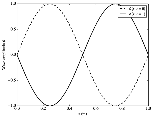
The solution field \(\phi\) at time \(t\) = 0 s and \(t\) = 1 s
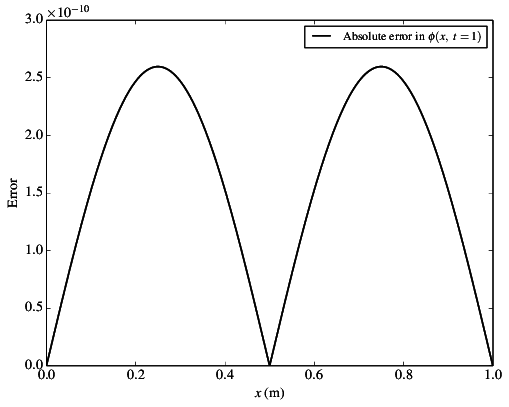
The error between the analytical solution and the numerical solution at time \(t\) = 1 s.